The Svedberg Number, 1.54, as the Basis of a State Function Describing the Evolution of Turbulence and Dispersion

Abstract

For natural flows, a definition equivalent to the Chezy-Manning mechanical equation is developed, but based on Coulomb interactions, which includes a state function that describes the evolution of tracer particles in turbulence. This makes it possible to overcome reductionist approaches (Navier-Stokes), which are limited by their complexity. This function shows the variation of the degrees of freedom of dispersion, as well as the statistical coupling of the solute with the flow, allowing to characterize very large or complex channels in “Dynamic Equilibrium.” An approach is also developed that links this function to universal constants of fractal motion.

1. Introduction

1.1 Definition of the “statistical sufficiency” of molecular phenomena

According to A. Annila et al. [1, 2] molecular systems at the macroscopic level, the statistical distribution of energy in these systems unfolds around the average molar thermal energy, R*To, (R as the gas constant, and To as the ambient Kelvin temperature) as shown in Figure 1.

Figure 1.

Energy distribution on a molecular system.

In “steady state,” (time invariant) oscillating particles are grouped into quantized energy zone (h*f) according to their probability. For the low-energy zone (E < RTo), many oscillators (blue) are grouped together but with low energy per unit; for the high-energy zone (E > RTo), only a few oscillators (red) will be able to supply the required high energy. In the central zone (E<RTo), close to the average value, there are enough oscillators with medium energy (green) in such a way that the sum of which is greater than in the low and high zones, with the highest probability.

In an open system, it is said to be “statistically sufficient” when the fluctuations around the mean (most likely) value are small, such that it does not change significantly, which is achieved if the “activation energy” is much lower than the average energy, W < <RTo.

1.2 Local equilibrium and “statistical sufficiency”: water fluidity and turbulent phenomena

The concept of local equilibrium in systems in non-thermodynamic equilibrium is essential for applying the usual thermodynamic equations to these systems, in which, despite not having “well-defined” variables such as temperature, energy, entropy, etc. there are well-defined “densities” of these variables, making it possible to analyze them consistently [3].

The validity of local equilibrium is limited by the ease with which dynamic processes restore “well-defined” initial distributions, in presence of fluctuations. In continuum mechanics, e.g., in hydrodynamics, when fluctuations act and the system tries to return to its “local” equilibrium, if the system in its dynamics suffers a non-linearity, e.g., the term v*grad (v) in the CM equation, the return to the previous point of local equilibrium is not possible because the results of the equation are not univocal, diversifying the behavior of the system. This effect of positive feedback is at the root of the problem of the “non-computability” of nonlinear phenomena (Figure 2) [4].

Figure 2.

Local equilibrium and fluctuations.

The range of validity of the local equilibrium in certain phenomena is not generally known from a microscopic perspective. However, it can be said that for gases, liquids, and transport phenomena, it exists well enough if the gradients of the intensive state variables are small and vary very slowly.

According to J. Frenkel in his “Kinetic theory of liquids” [5], due to the high fluidity properties of water—i.e., the capability of yielding a stress—this liquid allows for shear movements with almost no resistance. This behavior of water is measured by the ratio of the time, “τ” required to construct a population of “holes” in the lattice of liquid, to the basic period of atomic oscillation, τ_o ≈ 10⁻¹³ (sec).

$$\frac{\mathit{\tau }}{\mathit{\tau o}}\approx {\mathit{e}}^{\frac{∆\mathit{W}}{\mathit{RT}}}$$E1

This time τ is named the “half-life” of a particle in a “vacancy” position (hole) in the lattice of the liquid. If the ratio τ/τo is small, the fluidity of the liquid will be high, and if it is large, it will be low. Here, ΔW is the so-called “activation energy” in fluid, ΔW≈0.58 KJ/mol, being currently less than the maximum work of “forming a gap” in the water lattice, so, if the thermal heat is RT≈2.5 KJ/mol (at 300 K), then τ/τo ≈1.26, i.e., enough close to the ideal value of fluidity [3].

To define its state of “turbulence” in the case of water, the so-called “Reynolds Number” (Re) is used, which is the ratio between the product of a characteristic length, L, and the average velocity of the flow, U, and the “kinematic viscosity”, ν, which are dimensionally equivalent.

$$\mathit{Re}=\frac{\mathit{U}\ast \mathit{L}}{\mathit{\nu }}$$E2

The turbulence begins when U threshold is transposed, called the “critical” Reynolds Number (Rec), when nonlinearity also begins to occur at the microscopic level, but maintaining approximately the nature of “statistical sufficiency,” in which thermodynamic force (gradient of potential energy) quickly generates a flow (mass transport), without giving time for nonlinear phenomena to fully develop, thanks to its high fluidity.

Then, fluctuations, not so large, do not appreciably modify the energetic characteristic of the system. Water in turbulence, with velocities in a low and medium range, is “quite statistical,” i.e., the energy changes that occur will not significantly change the quasi-equilibrium condition, falling into the “Linear” regime of irreversible thermodynamics, in which the system evolves “slowly,” and the state remains stable (Figure 3).

Figure 3.

Regimes of thermodynamics.

2. Geomorphology and flow: factors that determine the behavior of natural streams, and the average velocity of the flow determines two important aspects of natural channels

2.1 Average velocity and geomorphology

The complex behavior of natural channels is marked by the role of flow velocity, both in the configuration of the geomorphology (profiles, geometry, and nature of the riverbed) and in the dynamics of the flow itself (distributions and values of the velocity vectors) [6]. This deep relationship is shown in the law of Conservation of Flow, in which the flow rate, Q, depends on the mean velocity, U, and the cross-sectional area of the flow, Ayz (Figure 4).

Figure 4.

Interaction of flow and geomorphology.

$$\mathit{Q}\approx \frac{\mathit{U}}{\mathit{Ayz}}$$E3

2.2 Average velocity and flow behavior

The average velocity not only interacts with the geomorphology but also with the flow itself. This is observed in the basic differential equation of point velocity, v, of NS equation [7], which depends on a nonlinear way of pressure, p, temperature, T, external forces, f, water density, ρ, and time.

$$\mathit{\rho }\left(\frac{\mathit{\partial v}}{\mathit{\partial t}}+\mathit{v}\ast \nabla \mathit{v}\right)=-\nabla \mathit{p}+\nabla \ast \mathit{T}+\mathit{f}$$E4

When the velocity value passes a threshold (Rec), the fluctuations by shear start to be amplified by nonlinearity and turbulence appears [8]. In this condition, the cross-sectional distribution of the longitudinal point velocity vectors is configured as a “Random Variable,” mainly described by the normal distribution, since the viscous rupture of the flows can be modeled as a bifurcation with two probable, symmetrical values, which are congruent with the measurement errors of the Gaussian bell [7].

This homogeneity in the results is reflected in the classical (Pr) distribution, which is essentially “flat” except at the edges due to the progressive effect of the viscosity of the boundary (Figure 5).

Figure 5.

Prandtl distribution of velocities.

2.3 Thermodynamic forces and flows of natural streams in the “linear” regime of irreversible thermodynamics. Convergence with the CM equation

Turbulent dynamics are composed of heterogeneous movements, usually rotational in nature, to expend free energy in the fastest way [9]. In the first stage, the strength of these movements is diminished by the great fluidity of the water, due to its nature of “statistical sufficiency.”

Then, for certain “normal” low range of velocities, this condition fundamentally allows turbulent flows to develop in the “linear” region of irreversible thermodynamics where thermodynamic “forces” (potential gradients) are linearly related with thermodynamic “flows” (mass or charge transport). This condition is examined for a natural flow as follows:

From the definitions of thermodynamic forces and flows, the following expressions can be established for natural flows, with ρ the water density, and U the mean velocity, obtaining the flow, J:

$$\mathit{J}\approx \frac{\frac{∆\mathit{m}}{\mathit{Ayz}}}{∆\mathit{t}}\approx \frac{\frac{∆\mathit{m}}{∆\mathit{Y}\ast ∆\mathit{Z}}}{∆\mathit{t}}\ast \frac{∆\mathit{X}}{∆\mathit{X}}\approx \frac{\left(\frac{∆\mathit{m}}{∆\mathit{V}}\right)\ast ∆\mathit{X}}{∆\mathit{t}}\approx \mathit{\rho }\ast \mathit{U}$$E5

For the Force, F, it holds, considering the potential energy gradient:

$$\mathit{F}\approx ∆\mathit{m}\ast \mathit{g}\ast ∆\mathit{h}\approx \frac{\left(∆\mathit{m}\ast \mathit{g}\ast ∆\mathit{h}\right)\ast ∆\mathit{X}}{∆\mathit{X}}\approx ∆\mathit{m}\ast \mathit{g}\ast \frac{∆\mathit{h}}{∆\mathit{X}}\ast ∆\mathit{X}\approx \mathit{\rho }\ast \mathit{Ayz}\ast \mathit{g}\ast \mathit{S}$$E6

Considering the basic relation of linear thermodynamics of irreversibility, force as cause and flow as a consequence:

$$\mathit{J}\approx \mathit{L}\ast \mathit{F}$$E7

Therefore, from (4), (5), and (6), in this case, the mean velocity of flow is proportional to the Slope S., if valid “linear” regime:

$$\mathit{U}\approx \mathit{L}\ast \left(\mathit{Ayz}\ast \mathit{g}\right)\ast \mathit{S}$$E8

It is now necessary to analyze the classical CM equation of flow in order to compare it with the previous result, in which “R” is the hydraulic radius, “n” is the opposition to the flow (Roughness), and “S” is the slope of the flow.

$$\mathit{U}\approx \frac{{\mathit{R}}^{\frac{2}{3}}}{\mathit{n}}\sqrt{\mathit{S}}$$E9

It is obvious that the mean velocity is not linear with the slope, but proportional to the square root of it. Now, it is interesting to establish the degree of “non-linearity” of CM Eq. (9) with respect to the thermodynamic Eq. (8) and compare the curves corresponding to each case (Figure 6).

Figure 6.

Linear fitting of Chezy-manning equation.

By separating the range of the slope into segments to compare √S with S, it can be verified that the blue curve (√S) can be linearized by lines that fit in each range, from 0–10%, with an approximate relative error of 10% in larger segment.

This result is compatible with a McLaurin-Taylor (Tl) series expansion for representative values [10]. So, it can be said that the classical equation of hydraulics corresponds well with a linear approximation on the slope and that therefore in the practical range of the slopes, the condition of thermodynamic “linearity” of the flow is approximately satisfied, compatible with the hypotheses proposed in this article. This may be called the “linearity approximation.”

2.4 The linear regime of irreversible thermodynamics and minimum entropy production. Effect of the “linearity approximation”

According to I. Prigogine, when both Forces and thermodynamic flows can be defined for an open system, their product is equal to the entropy production per unit volume, ΔiS/(dt*dV). [3], and also that the entropy, S, has a maximum (Figure 7).

Figure 7.

Behavior of entropy and entropy production.

Consistent with this situation, the distribution of probabilities in the volumes of the flow (according to Boltzmann’s concept) ideally tends to be a well-extended “coarse-grained” volume, [11] in which the microstates are indistinguishable. But actually, it is not “ideal,” considering that there is a (small) error for the “linearity approximation.” This special circumstance makes the “coarse-grained” areas have disseminated “gaps” that are detected as groups of more vigorous or more numerous fluctuations, showing the “intermittencies” that are observed experimentally in real flows (Figure 8).

Figure 8.

Effect of nonlinear fluctuations.

So, in the real case of turbulent water flow, it will be shown that the fluidity is low, but it is not zero, then it is necessary to consider the existence of “intermittences,” leading the “coarse-grained” regions painted with “patches” that are not representative of the ensemble, but being concordant statistically with PrN distribution. In this case, it is necessary to consider the velocity “Variance,” σ_u, that involves the deviations from the “linearity” of the turbulent phenomenon. An expression of measuring this parameter is proposed below (Figure 9).

Figure 9.

Variance as effect of non-linearities in flow.

$$\mathit{U}\left(\mathit{\text{measured}}\right)\approx <\mathit{U}>\pm {\mathit{\sigma }}_{\mathit{U}}$$E10

This parameter, σ_U, must be calculated not only in terms of purely hydraulic magnitudes since the dynamic equilibrium condition depends on a larger set of variables, which influence variance.

3. “Dynamic equilibrium” in the channels and “linear” region of the thermodynamics of irreversible processes

The linear region of irreversible thermodynamics is characterized by the fact that open systems that evolve in this regime ideally present “stable states,” that is, they do not vary with time, while their entropy production is a minimum, and thermodynamic flows tend to be constant, as is actually observed in natural waterways.

3.1 Basic characteristics of dynamic equilibrium in natural streams

The processes in natural turbulent streams establish a tendency for the flow to oscillate around a certain value of the flow state parameters, which is called “Dynamic equilibrium,” in that locally there are variations, but its state tends to stabilize (Figure 10).

Figure 10.

Dynamic equilibrium tends to steady state in flows.

Local variations are caused by contrary forces, and the point values are such that the energy and its distribution in its course take the most probable configurations, responding in detail to the following general criteria [12].

1. If river systems are in a “steady state” (invariant with time) due to the self-adjusting action of opposing forces, then the entropy of the open system, S, is the maximum possible, in congruence with the constraints imposed by the environment, and therefore the internal production of entropy, ΔiS/(dt), is the minimum possible.

2. At “dynamic equilibrium,” if the entropy production in the flow is the minimum possible and almost constant, the probabilities in the flow realm are ideally equivalent, this implies that the mass transport rates are ideally equivalent to each other, and concordant with the overall mean transport rate, leading to the fulfillment of the Prandlt distribution for the longitudinal velocities on the transverse axis of a river (Figure 11).

   $$\mathit{uj}\approx \mathit{uk}\forall \mathit{j}\mathit{\text{and}}\mathit{k}\mathit{U}\approx \frac{{\sum }_{\mathit{n}}\mathit{u}\left(\mathit{n}\right)}{\mathit{n}}$$E11

   The mean velocity is almost constant in all its course, as found by L. Leopold. Becoming very similar at birth to your delta, this is:

   u1<u2<u3<u4<u5<u6<u7<u8<u9<u10 (Figure 12) [13].

3. Under these conditions, the entropy production is equal to the product of the thermodynamic force and flow, with constant temperature and pressure, and no electric or magnetic fields.

Figure 11.

Local and general velocities in steady state.

Figure 12.

Leopold’s longitudinal continuity of velocity.

$$\mathit{Ps}\approx \frac{∆\mathit{\text{iS}}}{∆\mathit{t}}\approx \mathit{L}\ast \mathit{J}\ast \mathit{F}$$E12

In 2.2, F, the “Force,” is a gravitational gradient and J, the “Flow,” is the mass transport per unit of cross-sectional area and time.

4. Formation of the tracer plume in a turbulent flow, and models that represent its dynamic

4.1 Thermodynamic foundation of the phenomenon

Tracers are salt inks that solubilize in water, with a very limited environmental impact, presenting physical or chemical properties that allow their detection by instruments, such as their fluorescence or conductivity, which enables their widespread use for the scientific characterization of flows [14].

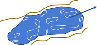
An injection of tracer into the flow configures the creation of a “plume” that advances as an open, isothermal-isobaric system, which breaks the chemical equilibrium in the system, implying in some way the reorganization of the internal molecular distributions.

When the solute is injected into the flow, two phases take place: A. SOLVATION in which the dipoles of the water act on the ions of the salt, separating them from the crystal structure, that is, working against the forces of interaction of the crystal lattice. B. DILUTION, which happens once the solvation of all the ions has been completed, and they are incorporated into the flow, moving with their own speed that depends on the concentration of the salt, which varies over time (Figure 13).

Figure 13.

Dye tracer salt dilution in streams.

The initial phase of SOLVATION is explained as the creation of hydrated ions (surrounded by water molecules), which must first be separated from the crystal lattice of the solid, and then electrically bonded to these molecules. This occurs because the energy of interaction between ions and dipoles destroys the crystal lattice.

This phase of the process, which is exothermic, decreases the potential energy of the whole so that the different particles are “ordered” better, which causes the entropy to decrease, which is expelled as heat to the outside.

This process may be interpreted as the battle and equalization of two opposing energies: the heat (enthalpy) of formation of crystal, and the heat of Solvation, given from the surrounding water (H₂0), whose two hydrogen atoms and one oxygen atom act as separate electric charges (dipoles), whose specific interactions are responsible for the destruction of the solid, giving ions.

The enthalpy of formation (positive), +ΔUo, of the crystal structure of the solid, and the Solvation heat (negative), -ΔHh, which is added to the salt from the water, its difference is the Dilution heat: T*ΔSd ≈ΔHd, which balance equation is as follow (Figure 14).

Figure 14.

Entropy expulsion in tracer system.

$$∆\mathit{Hd}\approx T\ast \mathit{\Delta iS}\approx ∆\mathit{Uo}-∆\mathit{Hh}$$E13

Thus, the joint action of ΔHh and ΔUo is spontaneous “internal” reorganizations in the system, which does not consume energy other than that shown in Eq. (13).

The next phase, called the DILUTION Phase, occurs when the generation of ions has ended when the solid structure of the solute is completely destroyed. At this point, it is necessary to consider the other interaction between the ions themselves, already in freedom, which are distributed forming an “ion cloud” that is a function of the Concentration, C(t) (Figure 15).

Figure 15.

Ion-ion interaction in tracer spreading [14].

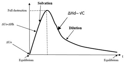
This phase, like the first one, involves a decrease in the potential energy of the whole, then it is also exothermic, with the expulsion of a spreading heat, ΔHd, which is now proportional to the square root of the concentration, √C, which decreases over time, as established in electrochemical thermodynamics (Figure 16).

Figure 16.

Thermodynamic process of a tracer in flow.

The interactions of the ions with each other reduce their mobility, which implies a “slowing down” effect on their movement. This effect is similar to the increase in friction by the Stokes mechanism.

Thus, for initial conditions (high concentration), the aggregate ions will have a small Stokes velocity, u1, for a medium concentration, they will have a higher velocity, u2, and in their final stage (low concentrations) their eigen velocity, u3, will be larger, equaling the velocity of the flow (Figure 17).

Figure 17.

Concentration affects the tracer velocity.

$$u1<u2<u3$$E14

And:

$$u3\approx U$$E15

This indicates that the transport time, ts, of the solute ions, depending on the decreasing concentration, will decrease as the effective velocity increases: ts1 > ts2 > ts3.

4.2 Advection-dispersion transport model

Although the transport of conservative substances in turbulent flows has been characterized by Fick’s equation, initially developed to represent diffusive motions associated with Brownian movement, G.I [15, 16]. Taylor postulated in 1954 that the main mechanism for the mixing of solutes in the flow is the “shear” effect, which can be represented also by these equations. In other words, this statistical movement is proportional to the concentration gradient. This effect corresponds to the longitudinal breakdown of the minimum parcels of the flow by the action of “separation” by the point velocity vectors, which are a random quantity.

This model is important in that it shows that the mean velocity, U, is composed of an infinite number of different components, that this velocity value is a statistical result of all its components, and that the magnitude of the DISPERSION (Longitudinal Coefficient of Dispersion, E) depends on the magnitude of the velocity.

$$E\approx f\left(U,\frac{\partial C}{\partial X}\right)$$E16

While LONGITUDINAL DISPERSION (lengthwise) is essentially determined by the shear effect of velocity, TRANSVERSE DIFFUSION (across width) is basically determined by turbulent mixing. This and other efforts to characterize the mixture of solutes in turbulence aim to describe and explain the curve in time of the tracer’s passage at a fixed point (Eulerian observer). Gathering all the knowledge, the equation of this curve has been established, according to the advection-dispersion model, which includes the average velocity and concentration in the cross-section of the flow, as functions of time and distance, Tl equation:

$$\frac{\partial C}{\partial t}+U\frac{\partial C}{\partial X}\approx E\frac{{\partial }^{2}C}{{\partial X}^2}$$E17

The solution of which is Fick’s equation, where Xo is the distance from sudden injection, M is the injected mass, and A_yz is the cross-section area.:

$$C\left(t,X\right)\approx \frac{M}{\mathit{Ayz}\sqrt{4\mathit{Et}}}{e}^{-\frac{{\left(\mathit{Xo}-U\ast t\right)}^2}{4\mathit{Et}}}$$E18

Numerous controversies have arisen regarding the shape of the bell-shaped (Gaussian) curve of the tracer’s response, since although it maintains a bias due to the Galilean composition of the velocity (Xo-U*t) that exists in the Neperian function, many times the experimental bias observed is greater than expected (Abnormal bias), and some discrepancies about the peak concentration (Figure 18).

Figure 18.

“Abnormal” biased tracer curve.

4.3 Transient storage (TS) and aggregated dead zone (ADZ) model for tracer evolution in flow

The TS Model has been proposed extending the classical advection-dispersion model but has been unable to adequately describe the abnormal bias in tracer curves [17, 18]. It assumes that there are “Storage zones” or areas that retain or trap groups of tracer particles on the periphery of the channel, which are subsequently released, affecting the longitudinal dispersion of the stream. The “Storage zones” are characterized by a proper concentration, Cs, where the solute is homogeneously distributed, and a volume defined by an area AS in the cross-section, while the central channel shows a concentration, Cb, and a volume defined by an area Ab. Between the two volumes, perimeter dead zone, and central channel, there is an exchange of particles, as already stated, defined by “α.” They are not considered chemical reactions or non-conservative changes in the solute (Figure 19).

Figure 19.

Dead zone storing tracer in borders.

The objective of the model is to calculate parameters, such as: As, Ab, α, and the longitudinal coefficient of dispersion, E, that can reasonably describe the actual tracer curve evolution, with its abnormal bias and peak concentration value.

An initial difficulty is that the model’s own equations (which add terms to the classical advection-dispersion equations) must be fitted (“calibrated”) by external software programs from data obtained from tracer experiments. This type of software is based on a “trial and error” procedure of the “Monte Carlo” type, which gives results with different settings, taking away the modeler’s own ability to analyze.

The “Aggregate Dead Zone” ADZ method, unlike the previous method, TS, uses first-order differential equations that directly link the parameters of interest. Its transport mechanism is based on conceptually separating advection from dispersion, assigning each characteristic of these a corresponding volume. The total volume of flow (V) is assigned to advection, and the fully mixed volume (Vm) is assigned to dispersion, maintaining the model of net “separation” between different zones of the channel. This model ADZ also uses computational software resources to fit the results as the previous model.

4.4 Some dynamic and thermodynamic problems of these models: Maxwell’s devil and null exergy for the process

In thermodynamics, “Work” is a macroscopic concept associated with the raising or lowering of a weight, the stretching or shortening of a spring [19], or any other means of transducing energy on a human scale, what O. Levenspiel [20] has called “axis work.” Fortunately, when chemical imbalance is studied (which is the case of dispersion in a flow), it can be considered thermal and mechanical equilibrium since a fluid medium will have the same temperature and pressures, which greatly simplifies its analytical treatment. This treatment can focus almost exclusively on the nature of particle distributions and the conditions that determine mass transport.

As stated, while the longitudinal dispersion is essentially due to the shear rupture in the fluid, the transverse diffusion (in Y Axis) is almost entirely due to the turbulent mixing, which, in addition to having a Fickian nature, can be developed analytically from an initial discontinuity of the “Dirac impulse” type (Figure 20).

Figure 20.

Abrupt cuts in concentration tend to smooth behavior.

This development shows that, regardless of whether initial conditions of discontinuity are imposed, as would be the case with the Dead Zones (or Storage Zones) and the Central Zone), the dynamics should always become a soft Fickian function. Any arbitrary cut that is made on the distribution always leads to smooth, monotonous solutions.

A non-natural distribution with abrupt changes, such as those proposed by the TS or ADZ model in peripheral zones, would be shown as follows (Figure 21).

Figure 21.

Maxwell‘s devil choosing slow particles.

This unnatural distribution would only be possible if a “Maxwell’s Demon” chooses only the slow particles, in the discontinuation of concentration, to store them. This, of course, would violate the 2nd Principle.

In this particular case, the only work that can be identified is that of frictional forces, so all the energy that goes into the system is spent on heat, and therefore the “available” energy for this spontaneous process of solvation-dissolution can be expressed as [20, 21]:

$$W\left(\mathit{\text{available}}\right)\approx T\ast ∆\mathit{\text{iS}}\approx 0$$E19

So, although the conceptual basis of this method is wrong, the operational time equations, obtained by software manipulation, are still useful in reactors and water quality studies.

5. A new vision of advection-diffusion. The state function that describes its evolution in turbulent flows

5.1 Nonlinear nature of molecular phenomena as a basic problem of physical models, and a macroscopic way of studying these processes

Nonlinearity, as an inevitable fact in physical reality, has been a permanent obstacle in the configuration of models of physical mechanisms [22], particularly those that attempt to describe molecular interactions in phase changes, such as those that occur in the formation of the tracer plume in a turbulent flow. In this process, there is a change from the solid state of the solute to a liquid state when it mixes with water.

The practical way to handle this problem has been to expand the nonlinear NS equation by means of numerical methods, whereas there are no general methods to solve it. This is because in this type of differential equation, main variables cannot be separated and cannot be identified separately [23]. This situation of “intractability” can be lessened if the “statistical sufficiency” condition of the system is met, and it is possible to identify and manipulate variables separately, such as thermodynamic flows and forces.

The microscopic non-predictability of the processes described by the nonlinear differential equation (that describes Poincare trajectories that collapse), can be overcome by a macroscopic thermodynamic analysis if the so-called “State Functions”, or “point function”, Φ(ε1,ε2) between two concrete states, ε1 and ε2, are used, since, as is known, despite the fact that the phenomenon is irreversible, nonlinear, (dotted lines) the evolution of this type of functions can be calculated by reversible (full lines) trajectories, in which the deviation from equilibrium is considered infinitesimal by devising ideal “quasi-static” processes as shown in Figure 22 [3, 24].

Figure 22.

Point function replacing nonlinear functions.

$${\int }_{\epsilon 1}^{\epsilon 2}\mathit{d\varphi }=\varphi \left(\epsilon 2\right)-\varphi \left(ϵ1\right)$$E20

This implies that, currently, although dynamic processes are “non-computable” at the differential level, “point functions” can be computed based on their initial and final macroscopic states. Nowadays [3], it is accepted that if temporal changes are used for the functions involved in the change from ε1 to ε2, under conditions of local equilibrium, it is feasible to calculate these functions on a “continuum” of time, restoring the analytical capacity on this type of events. State function then accomplishes the Schwartz condition if the system is on “statistical sufficiency.”

$$\oint \mathit{d\varphi }\left(t\right)\approx 0\text{if}W\ll \mathit{RT}$$E21

In this way, each pair of consecutive points of the “trajectories” is considered as the “beginning” and “end” of the elementary processes that compose it. In this way, a nonlinear evolution of the phenomenon can be represented by a continuous function that resolves such evolution.

5.2 Distributions in equilibrium. Svedberg’s constant in experiments on Brownian motion

In the first “linear” regime described in 2.2 [25, 26], thermodynamic equilibrium is basically characterized by the “Principle of detailed equilibrium” in which it is stated that “each identifiable physical process must be counteracted separately by its opposite” and is characterized by the independence (no interaction) of events, as established by the Poisson distribution. Such a representation is assigned to the initial observations of Brownian motion, as is analyzed below.

At the beginning of the twentieth century, the Swedish physicist T. Svedberg, in his investigations on the movement and distribution of colloidal particles seen under a microscope in an ultracentrifuge machine, verified the “Brownian motion” of such particles (Figure 23).

Figure 23.

Svedberg in front of his equipment [26].

These experiments, made on the count of colloidal particles on lattices observed from time to time, yielded very interesting numerical data, which were summarized statistically, in Table 1.

Number of particles, m	Cases of occurrence	Relative frequency	Poisson’s probability
0	112	0.216	0.214
1	168	0.325	0.330
2	130	0.251	0.254
3	69	0.133	0.131
4	32	0.062	0.050
5	5	0.010	0.016
6	1	0.002	0.004
7	1	0.002	0.001

Table 1.

Experimental and theoretical results of Svedberg observations.

The observed average value of this distribution, of # particles per unit of grid and per unit of time, <a>, is calculated as follows:

$$<a>\approx \frac{0\ast 112+1\ast 168+2\ast 130+3\ast 69+4\ast 32+5\ast 5+6\ast 1+7\ast 1}{518}\approx \frac{801}{518}\approx 1.546$$E22

This is the so-called “Svedberg number” [27], based on the distribution observed in the first two columns, and with the probabilities of occurrence, both from the combinatorial calculus (binomial distribution) and from the Poisson distribution, in accordance with the equilibrium (independence) assumption of the phenomenon.

5.3 Natural growth, geometric progression, and Brownian motion

For the Brownian motion, the total transport time will be described by the sum of a convergent series determined by the following differential equation, named “logistic curve, a nonlinear pattern with a development region and a saturation. This dynamic corresponds to a geometric convergence scaling, as in Figure 24 [22].

Figure 24.

Physical “law of growth.”

Focusing only on the “development” part, in which the growth differential is proportional to the growth itself, you can write:

$$\frac{\mathit{dr}}{r}\approx \int k\ast f\ast \mathit{dt}$$E23

Where “r” is the ratio between sequential quantities related to this transport, the solution of which is:

$$\mathrm{Ln}\left(r\right)\approx \int k\ast f\ast \mathit{dt}$$E24

The definition of the type of function “f” that is involved depends on the phenomenon that is being studied, for the case of Brownian motion, that function “f” would be a concentration of a solute, and “k” is the inverse of a remarkable time, T, we have for this the mean value <C > of Svedberg’s experiment, but in another context.

$$r\left(t\right)\approx e^{\frac{1}{T}\int C\left(t\right)\ast \mathit{dt}}\approx e^{<C>}\approx e^{1.54}\approx \left(1+<C>+\frac{<C{>}^2}{2!}+\dots +\frac{<C{>}^n}{n!}\right)$$E25

For the integral of (22), the ratio “r” corresponds to the division t/τ, where τ, as we know, is the basic (microscopic) time of the transport process and t is the total observation time. This solution is also identified with the “scale invariance,” hallmark of the Neperian function, implying a geometric growth over the value 1.54.

$$t\approx \tau \left(1+1.54+\frac{{1.54}^2}{2!}+..+\frac{{1.54}^n}{n!}\right)\approx \tau \ast 4.665$$E26

The value δ ≈ 4.669 appears as a “Universal Constant” in the work of M. Feigenbaum in 1975, [28] applying the concepts of “renormalization” that had been successful in the interpretation of nonlinear phase changes, understood that this technique, based strongly on the self-similarity of these phenomena, insofar as their description at different levels is mathematically identical, could be useful to apply to turbulence, in which there is a cascade of vortices that are included equally, one within the other. Considering an infinite process of bifurcations (period bending) for monomodal descriptions, strongly associated with the “logistic curve,” which describes in a simple way the processes of growth with losses.

Feigenbaum, for this case, found a “bifurcation tree” which, a constant of geometrical progression for the remarkable times, k, was coincident with that of Svedberg ratio:

$$\delta =\mathit{Lim}\frac{k_n-k_{n-1}}{k_{n+1}-k_n}\approx \frac{∆k\left(\mathit{\text{previous}}\right)}{∆k\left(\mathit{\text{posterior}}\right)}\approx 4.6692$$E27

5.4 Molecular basis of turbulence. Einstein’s mechanism and Svedberg’s constant

In his classic work on Brownian motion, A. Einstein [29] defined the sequential motion of molecular plots that move elementary distances, Δ, in a characteristic time, τ, in such a way that the mass transport described is in the condition of “statistical significance,” maintaining the mean thermal energy of dynamics.

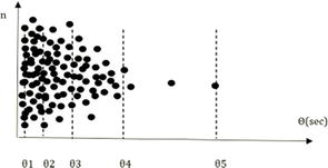
Then, a fixed Eulerian observer (blue) on the bank of a river, who measures the diffusion of a solute, will describe that as time passes, the arrival of sequential groups of solute molecules, each with a given concentration, n, as a function of time θn (Figure 25).

Figure 25.

Observer counting time arrivals of groups of tracer particles.

When the observer has done all the counting of the tracer particles, and the relationship (24) is established, it is possible to define a “diffusion velocity” such that: [30].

$$\mathit{vd}\approx \frac{\Delta }{\tau }$$E28

This expression can be extended according to Einstein’s definition, with D as the diffusion coefficient:

$$\mathit{vd}\approx \frac{\sqrt{2D\ast \tau }}{\tau }\approx \sqrt{\frac{2D}{\tau }}$$E29

Note that in this definition we should use not time as the general variable, “t,” but the “characteristic time,” τ, since we are describing molecular proper motions in the condition of “statistical significance,” which must, by definition, be shorter than the independent variable.

5.5 The state function Φ (U,D,t) that describes the evolution of the solute in the turbulent flow: the modified advection-diffusion equation

Since the phenomenon of dispersion depends to a large extent on the breakdown effect generated by advection, inversely proportional to the mean velocity, U, an evolution function, Φ (U,D,t) can be defined as follows:

$$\Phi \approx \frac{\mathit{vd}}{U}\approx \frac{\left(\frac{∆}{\tau }\right)}{U}\approx \frac{\sqrt{\frac{2D}{\tau }}}{U}$$E30

This function can also be developed as shown, with σ_t as the temporal variance of the Tl distribution of the tracer. Here 2.16 ≈ √δ.

$$\Phi \approx 2.16\ast \left(\frac{{\sigma }_t}{\mathit{tp}}\right)$$E31

From Eq. (30), you can find a modified version of Fick’s basic definition, nonlinearity (16), which fulfills representing the experimental tracer curves, without using the fallacious arguments of the TS or ADZ method:

$$C\left(t,X\right)\approx \frac{M}{Q\ast \Phi \ast t\ast 1.16}{e}^{-\frac{{\left(\mathit{tp}-t\right)}^2}{2\ast 0.214\ast {\left(\Phi \ast t\right)}^2}}$$E32

From this equation, with the solute mass, taking the peak value of the concentration and time, and the state function for that time, we can calculate the flow rate, Q:

$$Q\approx \frac{M}{\mathit{Cp}\ast \Phi \ast \mathit{tp}\ast 1.16}$$E33

Also, using the modified Fick function, but as a function not of time but of distance, the cross-sectional area of the flow, Ayz, can be calculated with the plotter, using a multiplier by 1000 in the denominator to fit the units.

$$\mathit{Ayz}\approx \frac{M}{1000\ast {\int }_{x1}^{x2}C\left(X\right)\mathit{dX}}$$E34

That is, it can be applied to describe nonlinear phenomena, such as turbulence, without having to solve the analytical problems associated with the NS equation. The curve representing Φ as in Figure 26 is proportional to the curve of the thermodynamic evolution of solute advance in Figure 16.

Figure 26.

State function curve as behavior curve.

In the dispersion stage, both solute ions and solvent (water) molecules are mixed in flow, and distributed in ever-increasing volumes, until when Φ ≈ 0.38, condition of “complete mixing” (homogeneous distribution of the tracer in the cross-section of the flow), when the velocity of the ions is almost that of the flow itself, according to Figure 17.

This is important because it allows you to have an analytical function that describes turbulence, without resorting to NS-type functions.

A practical definition of the state function, which is useful for calculations in the turbulence stage is as follows, with “M” the mass of the tracer, “Q” the discharge, “tp” is the peak time of solute distribution, and “γ” a constant that depends on the type of solute:

$$\Phi \approx \frac{M}{Q\ast \gamma \ast 1.16}\ast \frac{1}{\sqrt[3]{\mathit{tp}}}$$E35

Also, it is valid the following equation:

$$\mathit{Cp}\approx \gamma \ast {\mathit{tp}}^{-\frac{2}{3}}$$E36

Using these equations, we can write the following equation:

$$\Phi \approx \frac{M}{Q\ast {\gamma }^{3/2}\ast 1.16}\ast \sqrt[2]{\mathit{Cp}}$$E37

This result is coincident with the well-known behavior of ejected exothermal heat of solute in Figure 16.

On the other hand, one can, of course, equate the one-dimensional CM definitions (8) with Newtonian interactions, and the relation from Φ with Van-der Waals (electrical) dispersal interactions.

$$\frac{R^{\frac{2}{3}}}{n}\ast \sqrt{S}\approx \frac{1}{\Phi }\ast \sqrt{\frac{2D}{\tau }}$$E38

From this relationship, it is possible to establish the hydraulic variance as a function of the dispersive variance, and also calculate both hydraulic and dispersive magnitudes knowing values of Φ. This paves the way for the measurement of large streams, which is impossible to do with the state of the art.

$$\sigma \left(\mathit{\text{hydraulic}}\right)\approx f\left(\sigma \left(\mathit{\text{dispersive}}\right)\right)$$E39

In this way, the state function allows you to look precisely into the dynamics of turbulent flow, insofar as it can be calculated, U, Q, Ayz, y D, which is facilitated by the “Dynamic Equilibrium” condition of the channel, which presents large volumes in the condition of “Coarse grained” with nonlinear “patches,” which can be represented by σ_u (Figure 27).

Figure 27.

State function allows large river measurements.

6. Power function from the state function, which describes the ratio of notable numbers in dispersion and turbulence

It is interesting to see how the notable Feigenbaum numbers and the Golden Number are distributed in a certain order with respect to dispersion and turbulence, as power function of Φ (k) (Figure 28).

Figure 28.

Power function of Φ(k) [31].

This arrangement can be interpreted in that once dispersion begins, a relationship is established between the characteristic time, τ, and the general time, tp (by means of δ). Then, the relative, sequential vigor of the fluctuations is determined by the constant α. Finally, the rotational dynamics of the turbulence are established by the Golden Number, ψ, which establishes the vortices by Fibonacci scaling [31, 32].

7. Conclusions

1. The physical model analyzed here shows that turbulence, for practical purposes, can be looked at from a different point of view than the reductionist scheme of nonlinear partial differential eqs. (NS).

2. Tracers are fluorescent marker salts, which, when dissolved in natural flows, allow the characterization of heterogeneous movements of water, since these movements are the same as those of the solute molecules.

3. The great fluidity of water means that the usually “violent” movements of turbulence can be encased in the “linear” region of irreversible thermodynamics, where the “forces” (gradients) and the “flows” (rates of mass transport) are proportional, and the condition of “statistical sufficiency” is maintained, thanks to the fact that the “activation energy,” ΔW, is much less than thermal energy, RT.

4. It is shown how the use of “thermodynamic potentials,” in this case, a function of state, Φ, which is proportional to the enthalpies put into play, of “solvation” (when injecting the tracer), and of “dilution” as this cloud evolves, it is possible to obviate the difficult application of the NS equation, to obtain useful data in natural channels that are in “Dynamic equilibrium”.

5. In the definition of Φ, the “Svedberg constant,” a ≈ 1.54, which is the fractal hallmark of diffusive, Brownian, processes, plays an important role, allowing the calculation of the main variables in all types of channels.

6. In this paper, it is shown that the state function is proportional to square root of concentration, √C, as is expected from classical thermodynamics of solute evolution in flow.

7. It is possible to establish a power function that encompasses a sequence of the remarkable numbers that govern the fractal nature of turbulence.

Acronyms list

NS	navier-stokes
Re	reynolds number
Rec	critical reynolds number
Pr	prandtl
CM	chezy-manning